Setting up a basic environment in Genesis

I. Prerequisites

Python: 3.9+
OS: Linux (recommended) / MacOS / Windows (not recommended yet)

II. Installation

It is recomended that you set up some form of virtual environment before working on installing all the dependencies to follow the guide below. A simple venv should suffice, if you don’t want to have to install conda. The most stable version so far is Python 3.10 according to my experience.

Install PyTorch following the official instructions.
Install Genesis:

pip install genesis-world

If you need extra ability such as motion planning, surface reconstruction, and ray tracing please visit here for extra information

To check that you have installed everything correctly, run:

python -c "import genesis; print(genesis.__version__)"

You should see a result of version being returned (0.2.1 as of the date written)

III. Basic set up

We will now proceed to load a basic scene that render the model of an Unitree G1 robot. First, let’s create a working folder:

mkdir robot_demo
cd robot_demo

Then, clone the following repository so that we have access to all of the G1 mesh and description:

git clone https://github.com/janhq/robot-models.git

Alternatively, you can also find your own model. In this guide, we will only focus on urdf and mjcf (which use .xml extension) format. If you find any model that you would want us to add the repository above, please feel free to make a request!

Once that is done, we can create and open our main.py.

First, we will import all the necessary library:

import numpy as np
import genesis as gs
import json

Then, we will initialise the environment and create a base sim as follow:

gs.init(
    backend = gs.gs_backend.gpu, # it will automatically pick up your system gpu
    # change to below if you want to run on cpu
    # backend = gs.gs_backend.cpu
 
    precision = "32", # floating point precision
)
 
scene = gs.Scene(
    viewer_options = gs.options.ViewerOptions(
        camera_pos    = (3, 0, 2.5), # the position of the camera physically in meter
        camera_lookat = (0.0, 0.0, 0.5), # the position that the camera will look at
        camera_fov    = 40,
        max_FPS       = 60,
    ),
    sim_options = gs.options.SimOptions(
        dt = 0.01, # time change per step in second
    ),
    show_viewer = True, # whether or not to enable the interactive viewer
)
 
plane = scene.add_entity(
    gs.morphs.Plane(), # Add a flat plane for object to stay on
)

Next, we will add the robot model into the scene as follow:

root_path = "robot_models/unitree/g1/torso_only/"

1. For MuJoCo format (`.xml`), we do:

g1 = scene.add_entity(
    gs.morphs.MJCF(
        file = root_path + "g1_dual_arm.xml",
    )
)

2. For URDF format (`.urdf`), we do:

g1 = scene.add_entity(
    gs.morphs.URDF(
        file = root_path + "g1_dual_arm.urdf",
        fixed = True, # enable this if you want the main body to fix to a position
    )
)

And finally, we can build the scene:

scene.build()

Next, we will set up some parameter for the robot joint. In this guide, to keep it simple, we will only control the left arms. If you want to be able to control more, you can refer to the information regarding joint name and their angle range in the desc folder of the respective robot model.

with open(root_path + "desc/g1_dual_arm_<model-type>_config.json", 'r') as f:
    model_data = json.load(f)
 
l_arm_jnt_names = [ # refer to the markdown for a full list of joint name
    "left_shoulder_pitch_joint",
    "left_shoulder_roll_joint",
    "left_shoulder_yaw_joint",
    "left_elbow_joint",
    "left_wrist_roll_joint",
    "left_wrist_pitch_joint",
    "left_wrist_yaw_joint",
]
 
# convert name into index number for ease of control
l_arm_dofs_idx = [g1.get_joint(name).dof_idx_local for name in l_arm_jnt_names]
 
g1.set_dofs_kp( # set the proportional gain which determines the force joint use to correct its position error 
                # higher means more rigid
    kp=np.array([500] * len(l_arm_jnt_names)),
    dofs_idx_local=l_arm_dofs_idx,
)
 
g1.set_dofs_kv( # set the derivative gain which determines the force joint use to correct its velocity error
                # higher means more damping
    kv=np.array([30] * len(l_arm_jnt_names)),
    dofs_idx_local=l_arm_dofs_idx,
)
 
g1.set_dofs_force_range(  # refer to the json for more information
    lower=np.array(
        [model_data["joints"][name]["limits"]["force"][0] for name in l_arm_jnt_names]
    ),
    upper=np.array(
        [model_data["joints"][name]["limits"]["force"][1] for name in l_arm_jnt_names]
    ),
    dofs_idx_local=l_arm_dofs_idx,
)

Now that we are done with the set up, we will proceed to the last step which is running the simulation and see it render in an interactive viewer. This part is different for each OS so please follow the respective instruction below:

1. Linux

g1.set_dofs_position( # set the initial position of the joints
    np.array([0]*7), # all 7 joint angle is set to zero
    l_arm_dofs_idx,
)
 
# PD control
for i in range(200): # effectively 2 seconds of simulation
    if i == 100:
        g1.control_dofs_position( # control the robot to set the angle of each joint 
            np.array([-1, 0, 0, 0, 0, 0, 0]), # pitch to 1, the rest to 0 in radian
            l_arm_dofs_idx,
        )
 
    scene.step() # step through the simulation, each step is advance dt amount of time

2. MacOS (Tested on M series and above)

def run_sim(scene):
    g1.set_dofs_position( # set the initial position of the joints
        np.array([0]*7), # all 7 joint angle is set to zero
        l_arm_dofs_idx,
    )
 
    # PD control
    for i in range(200): # effectively 2 seconds of simulation
        if i == 100:
            g1.control_dofs_position( # control the robot to set the angle of each joint 
                np.array([1, 0, 0, 0, 0, 0, 0]), # pitch to 1, the rest to 0 in radian
                l_arm_dofs_idx,
            )
 
        scene.step() # step through the simulation, each step is advance dt amount of time
 
gs.tools.run_in_another_thread(fn=run_sim, args=(scene,))
 
if scene.visualizer.viewer is not None:
    scene.visualizer.viewer.start()

3. Windows (Not tested)

IV. Running the simulation

We can finally run the simulation by simply do:

python main.py

You should be able to see the FPS log in the terminal. You should also see a window pop up with the appropriate render of the robot. It should looks something like below.

g1 render

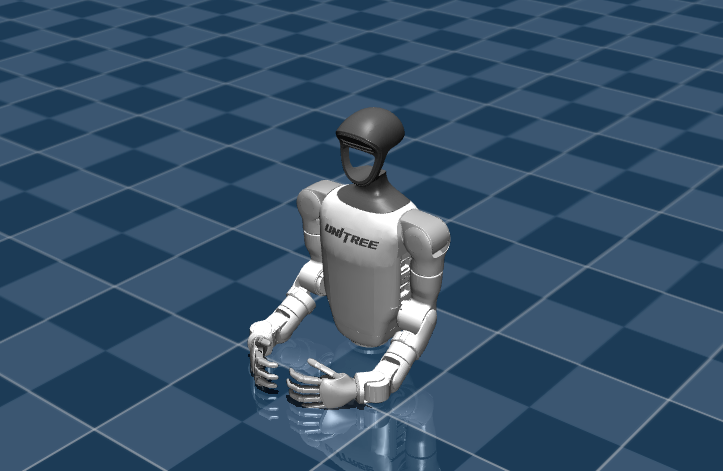
At timestep 100 (or after 1 second), you should be able to see the robot raise its left hands up. That is because remember that previously, we have controled the pitch of the shoulder to -1 radian.

And that concludes a basic set up of a simulation environment in Genesis.

Next, we will learn how to control each of the individual joint using keyboard inputs.

Ultimate Guide to Local Inference Controlling individual robot joint using keyboard